Statistics:
Types of data:
|
Categorical: |
Qualitative |
|
- Nominal |
· Labelled ·
No quantity or order |
|
- Ordinal |
· Numbered ·
Variable increments |
|
Numerical: |
Quantitative |
|
- Discrete |
·
Whole numbers only |
|
- Continuous |
· Any value · Constant increment · Interval data: false zero point (i.e. 20°C isn’t twice as hot as 10°C) · Ratio data: true zero point (e.g. 2/52 is twice as old as 1/52) |
Test selection:
|
|
2 groups |
>2 groups |
||
|
Paired |
Unpaired |
Paired |
Unpaired |
|
|
Parametric |
Student T |
Student T |
ANOVA |
ANOVA |
|
Non-parametric -Nominal |
McNemar |
Chi |
Cochrane Q |
Cochrane Q |
|
Non-parametric -Ordinal / ratio |
Wilcoxon Rank Sum |
Mann Whitney U |
Friedman |
Kruskell Wallis |
N.B. Parametric tests are used when data a) are numerical b) follow a distribution
Measures of central tendency:
|
Mean |
· Sum / number of observations · More affected by outliers |
|
Median |
· Half the observations are higher, other half are lower · Less affected by outliers |
|
Mode |
· Most frequently occurring value · Rarely relevant |
Measures of spread:
|
Inter-quartile range |
· Middle 50% of observations · Often represented on box and whisker plot o Box: 25, 50 and 75 o Whiskers: 10 and 90 |
|
Standard deviation |
· SD = √variance ·
Variance = ε(x-ẋ)2/(n-1), where |
|
Standard error |
·
SE = SD/√n, where · Indicates how far the sample mean is likely to be from the true mean · Used to derive confidence interval |
|
Confidence interval |
·
CI = mean ± z(SD/√n) · Indicates a range within the true value is likely to fall · Indicates both magnitude and certainty of difference (cf. P value) · If the confidence interval crosses 1.0, result is insignificant · Can be calculated for anything: mean, odds ratio, relative risk etc |
Comparisons:
Example:
|
|
Pain |
No pain |
|
Fentanyl |
A |
B |
|
Nothing |
C |
D |
|
Relative risk |
· Risk of pain in fentanyl group = A/(A+B) = RF · Risk of pain in nothing group = C/(C+D) = RN · Relative risk = RF/RN · The risk of the event in the intervention group compared with the risk of the even in the control group” · Amplifies the apparent effect of a drug on rare outcomes o e.g. if 1% to 0.3%: RRR is 70%, ARR is 0.3% |
|
Odds ratio |
· Odds of pain in fentanyl group = A/B = OF · Odds of pain in nothing group = C/D = ON · Odds ratio = OF/ON · “A ratio of event to non-event in the intervention group compared with the control group” · Almost the same as RR if large data set and rare event |
|
Hazard ratio |
· Hazard ratio is the relative risk of an event happening at time t · i.e. risk of pain now cf. risk of pain at some point |
|
Number needed to treat |
· Absolute risk reduction = RN - RF · NNT = 1 / (absolute risk reduction) |
Uncertainty:
|
Type 1 error |
· False positive ·
Threshold (α value) usually set 5% |
|
Type 2 error |
· False negative ·
Threshold (β value) usually set at 20% |
|
Power |
· The ability to detect a difference if there is one · Power = 1 – β value = usually 80% Determinants: · Sample size (for 2x precision, need 4x numbers) · Magnitude of difference · Threshold for effect · (many others) |
|
P value |
· Probability of finding this result (or greater) by chance if the null hypothesis were true · i.e. probability of this being a false positive result Problems with p = 0.05 · No account of prior probability · No indication of effect size · Not low enough if the stakes are high · Inappropriate for multiple comparisons (see Bonferroni correction) |
|
Fragility index |
· Number of patients whose change in status would turn a significant result into a non-significant result |
|
Bonferroni correction |
· Used if assessing for several outcomes simultaneously · Divide α (p = 0.05) by the number of tests being performed |
|
Rule of 3’s MCQ |
· If no events in the entire population, 95% confidence interval is <3 · Applies no matter how many in the population · Derived from binomial theory |
Screening vs diagnostic tests:
|
|
Screening |
Diagnostic |
|
Target |
Everyone |
Symptomatic; or Positive screening test |
|
Nature |
Non-invasive |
Invasive |
|
Thresholds |
High sensitivity (few false neg) |
High specificity (few false pos) |
|
Cost |
Cheap |
Expensive |
Screening tests: table
|
|
Difficult ETT |
Not difficult ETT |
Predictive values: |
|
High MP score |
a)True +ve |
b)False +ve |
PPV: a/(a+b) |
|
Low MP score |
c)False -ve |
d)True -ve |
NPV: d/(c+d) |
|
|
Sensitivity: a/(a+c) |
Specificity: d/(b+d) |
|
|
|
|
|
|
|
|
· Positive LR = sensitivity / (1-specificity) · Negative LR = (1-sensitivity) / specificity |
|
|
|
|
|
||
Screening tests: definitions
|
Sensitivity |
· If have disease, how likely is the test to agree · SNOUT: SeNsitive test when negative rules OUT the disease |
|
Specificity |
· if don’t have disease, how likely is the test to agree · SPIN: a SPecific test when positive rule IN the disease |
|
PPV |
· If test says yes disease, how likely to have disease · ∝ prevalence as well as test quality |
|
NPV |
· If test says no disease, how likely to not have disease · ∝ rareness as well as test quality |
|
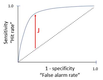
Receiver operator characteristic |
· Relationship between sensitivity, specificity, test quality · ↑AUC associated with high utility
|
|
Youden’s J statistic |
· J = sensitivity + specificity - 1 · J = point of maximum divergence of the curve · Single representation of a test’s utility, between 0 to 1 |
Feedback welcome at ketaminenightmares@gmail.com